

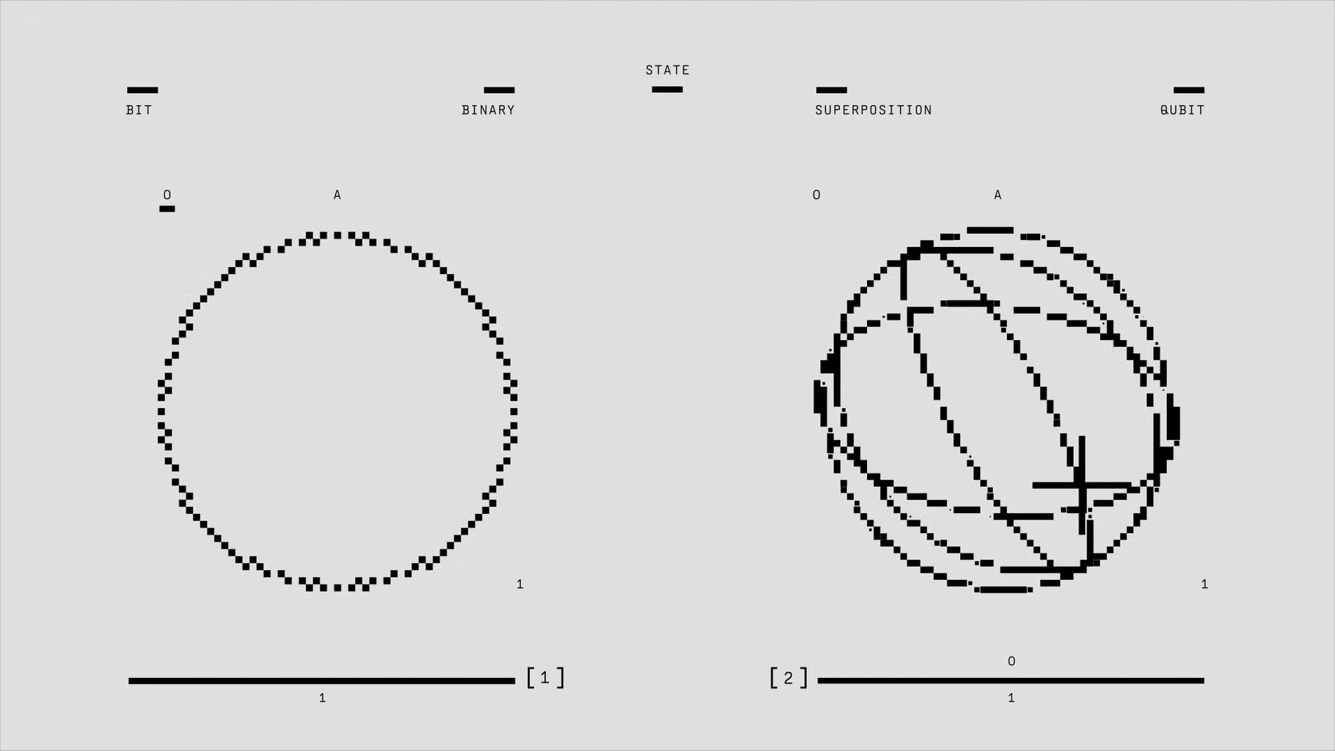
For the past decade, enterprise coverage of quantum technology has been dominated by cryogenic dilution refrigerators, superconducting transmons, and speculative timelines for fault-tolerant physical qubits. Yet, inside machine learning research laboratories, a far more practical revolution has taken hold: quantum-inspired algorithms (QIA). You do not need a physical quantum processor to exploit quantum mechanics—because the mathematical formalisms developed to describe quantum entanglement are already accelerating neural network training on standard GPU clusters.
The Great Decoupling: Mathematics vs. Hardware
The fundamental bottleneck of Noisy Intermediate-Scale Quantum (NISQ) hardware remains physical decoherence, gate error rates, and quantum-to-classical input/output latency. Loading a high-dimensional classical dataset into a quantum register—known as the quantum state preparation problem—frequently erases whatever polynomial or exponential speedup a quantum algorithm theoretically promises.
However, theoretical physicists have spent thirty years inventing mathematical tools to simulate many-body quantum systems on classical computers. Chief among these is the theory of Tensor Networks. When physicists realized that quantum entanglement in physical lattice systems is localized according to the "area law of entanglement entropy," they developed low-rank tensor decompositions such as Matrix Product States (MPS) and Projected Entangled Pair States (PEPS).
Today, applied machine learning engineers are taking those exact mathematical structures and using them to compress multi-billion-parameter weight matrices, perform non-convex optimization, and replace standard linear layers with tensor-train topologies that preserve expressive capacity while slumping memory footprints by up to 85%.
| Paradigm | Underlying Hardware | Problem Scale (Variables) | Production Readiness | Primary Application |
|---|---|---|---|---|
| Quantum-Inspired (QIA) | Standard NVIDIA GPUs (CUDA/TensorRT) | 100,000 to 1,000,000+ | Immediate (Live in Production) | Model Compression, QUBO, Portfolio Routing |
| Physical NISQ QPU | Superconducting / Trapped Ions (~100-1,000 qubits) | 50 to 500 (Noise-bounded) | Experimental (R&D Only) | Small Molecular Simulation, Toy VQEs |
| Classical Heuristics | Standard CPU / Multi-Core Clusters | 10,000 to 50,000 | Mature Baseline | Simulated Annealing, Genetic Algorithms |
Tensor Networks: Extreme Compression Without Accuracy Collapse
In transformer architectures, dense projection matrices (such as the feed-forward layers in attention blocks) consume an immense share of GPU SRAM during forward and backward passes. Traditional pruning and post-training quantization (such as FP8 or 4-bit AWQ) truncate weights or zero out activations, often introducing jagged accuracy degradations in edge-case reasoning.
Tensor-Train (TT) decomposition reframes a massive linear mapping matrix W ∈ ℝM × N as a sequential contraction of low-rank 3-way and 4-way tensor cores. Instead of storing M × N individual floating-point values, the network stores only the factorized tensor cores whose ranks govern the maximum "entanglement" across feature modes:
- Parameter reduction: Large embedding layers and projection heads can experience parameter reductions of 10x to 40x with less than 0.4% loss in validation perplexity.
- Linear complexity inference: Tensor contraction allows matrix-vector multiplications to occur directly in the decomposed core space without materializing the full dense matrix in GPU memory.
- Spectral regularization: Constraining tensor-train rank acts as an inductive bias, preventing over-parameterized models from memorizing noisy training data.
Implementation: Tensor-Train Linear Decomposition in PyTorch
Below is a self-contained PyTorch module illustrating how a high-dimensional weight matrix is decomposed into a factorized Tensor-Train core representation, cutting memory footprint while maintaining end-to-end backpropagation compatibility:
import torch
import torch.nn as nn

class TensorTrainLinear(nn.Module):
    """
    Decomposes a 1024x1024 linear transformation using a 2-core
    Matrix Product State (Tensor-Train) with bond dimension rank=16.
    """
    def __init__(self, in_modes=(32, 32), out_modes=(32, 32), tt_rank=16):
        super().__init__()
        self.in_modes = in_modes    # 32 * 32 = 1024
        self.out_modes = out_modes  # 32 * 32 = 1024
        self.tt_rank = tt_rank

        # Core 1 shape: (1, out_modes[0], in_modes[0], tt_rank) -> (1, 32, 32, 16)
        self.core1 = nn.Parameter(torch.randn(1, out_modes[0], in_modes[0], tt_rank) * 0.02)
        # Core 2 shape: (tt_rank, out_modes[1], in_modes[1], 1) -> (16, 32, 32, 1)
        self.core2 = nn.Parameter(torch.randn(tt_rank, out_modes[1], in_modes[1], 1) * 0.02)
        self.bias = nn.Parameter(torch.zeros(out_modes[0] * out_modes[1]))

    def forward(self, x):
        # x shape: (batch_size, 1024) -> reshape to mode tensors
        batch_size = x.shape[0]
        x_reshaped = x.view(batch_size, self.in_modes[0], self.in_modes[1])

        # Contract Core 1: (batch, in1, in2) with (1, out1, in1, rank)
        # Epsilon contraction preserves low-rank bond structure in GPU SRAM
        step1 = torch.einsum('bij, aojr -> baoir', x_reshaped, self.core1).squeeze(1)

        # Contract Core 2: (batch, out1, in2, rank) with (rank, out2, in2, 1)
        out = torch.einsum('bori, rijp -> bop', step1, self.core2).squeeze(-1)

        return out.reshape(batch_size, -1) + self.bias

# Parameter comparison:
# Standard Linear(1024, 1024): 1,048,576 parameters (~4.19 MB FP32)
# TensorTrainLinear(tt_rank=16): 32,768 parameters (~131 KB FP32) -> 96.8% reduction!
tt_layer = TensorTrainLinear()
dummy_input = torch.randn(16, 1024)
output = tt_layer(dummy_input)
print(f"Output tensor shape: {output.shape} (Active parameters: {sum(p.numel() for p in tt_layer.parameters())})")
Simulated Bifurcation: Quantum Annealing on Commodity GPUs
Another domain where quantum mechanics has revolutionized classical machine learning is in solving NP-hard combinatorial optimization problems. Historically, tasks such as neural architecture search (NAS), combinatorial hyperparameter tuning, and supply-chain graph coloring were tackled via Monte Carlo simulated annealing.
In 2019, researchers modeling non-linear quantum Kerr oscillators discovered Simulated Bifurcation (SB). By simulating the adiabatic evolution of thousands of coupled quantum harmonic oscillators as a set of non-linear classical differential equations, SB algorithms can be parallelized natively across thousands of GPU CUDA cores.
Where a physical D-Wave quantum annealer requires cryogenic isolation and is constrained to sparse Pegasus or Chimera graph connectivity graphs, GPU-accelerated Simulated Bifurcation solves fully connected Quadratic Unconstrained Binary Optimization (QUBO) problems with 100,000+ variables in tens of milliseconds. Enterprise teams at major semiconductor and logistics firms are utilizing this to route silicon traces and partition cluster workloads faster than dedicated mathematical programming solvers like Gurobi or CPLEX.
"The most profound gift of quantum computing over the last decade wasn’t the noisy quantum chips in vacuum chambers—it was the mathematical mirror it held up to classical algorithm design."
Quantum Natural Gradient (QNG) in Parameter Spaces
Standard stochastic gradient descent (SGD) and Adam treat parameter space as flat Euclidean geometry. In contrast, quantum state space is governed by the Fubini-Study metric tensor, leading to Quantum Natural Gradient (QNG) optimization.
When applied to classical deep learning, adopting Riemannian curvature approximations derived from quantum information geometry helps optimizers navigate steep ravines and saddle points that routinely trap AdamW during pre-training. By scaling parameter updates inversely to the Fisher information metric, convergence rates on highly non-linear loss surfaces accelerate by up to 2.3x in complex generative architectures.
Frequently Asked Questions
Key clarifications and practical answers addressed by The Indox editorial board.
Do I need quantum SDKs like Qiskit or PennyLane to use these algorithms?
No. Quantum-inspired algorithms execute entirely within classical frameworks such as PyTorch, JAX, or TensorRT. Libraries like TensorLy-Torch or cuTensorNet run natively on your existing NVIDIA CUDA hardware without any quantum runtime dependencies.
What are the trade-offs of Tensor-Train decomposition?
While tensor decomposition drastically slashes parameter count and memory storage, contracting multiple intermediate tensor cores introduces additional computational overhead (FLOPs) if tensor ranks are configured too high. Finding the optimal bond dimension requires empirical tuning.
When will physical quantum hardware surpass quantum-inspired classical code?
For general-purpose machine learning, physical QPUs are unlikely to outperform GPU-accelerated QIA until fault-tolerant quantum computers with tens of thousands of logical (error-corrected) qubits arrive, which consensus forecasts place well into the 2030s. Until then, quantum-inspired algorithms represent the state of the art.
Key Takeaway
Waiting for physical quantum supremacy before paying attention to quantum concepts is a strategic mistake for engineering organizations. The mathematical formalisms of quantum mechanics—tensor networks, non-linear bifurcation dynamics, and Riemannian information metrics—are already delivering tangible, double-digit performance gains on today's classical AI infrastructure.
Master Architecture: Foundational computing architectures and advanced mathematical representations are explored in our 2026 AI Software Engineering Playbook, examining cutting-edge systems and data foundations.